In this post I’ll present some theory and Python code for solving ordinary differential equations numerically. I’ll discuss Euler’s Method first, because it is the most intuitive, and then I’ll present Taylor’s Method, and several Runge-Kutta Methods. Obviously, there is top notch software out there that does this stuff in its sleep, but it’s fun to do math and write programs. This material is adapted from the excellent textbook by Burden and Faires, Numerical Analysis 8th Ed., which is easily worth whatever they’re asking for it these days.
Euler’s Method
Although Euler’s method is seldom used in practice any longer, it is a great introduction to computational mathematics. We will use it to solve a single variable, ordinary differential equation of the form,
(1) ![]()
The differential equation describes how the derivative of ![]() behaves, as a function of an independent variable,
behaves, as a function of an independent variable, ![]() , and the function
, and the function ![]() . We would like to determine the function
. We would like to determine the function ![]() for the initial condition
for the initial condition ![]() , on the domain
, on the domain ![]() .
.
Euler’s method divides the domain into ![]() pieces of size
pieces of size ![]() . If the domain is given by
. If the domain is given by ![]() , then the step size is given by
, then the step size is given by ![]() .
.
The method then uses the derivative to approximate the the next value of the underlying function. Recall that the derivative of a function ![]() is given by,
is given by,
(2) ![]()
Since we will assume that ![]() is small, but not arbitrarily small, we’ll drop the equality. If we multiply both sides by
is small, but not arbitrarily small, we’ll drop the equality. If we multiply both sides by ![]() , then the denominator disappears and we obtain,
, then the denominator disappears and we obtain,
(3) ![]()
If we then add ![]() to both sides we obtain an approximate expression for the next value of
to both sides we obtain an approximate expression for the next value of ![]() ,
,
(4) ![]()
If we flip the equation around and replace ![]() and
and ![]() with
with ![]() and
and ![]() , respectively, then we obtain something that looks a little bit more like a line from a computer program,
, respectively, then we obtain something that looks a little bit more like a line from a computer program,
(5) ![]()
We can then write the method more succinctly as,
(6) ![]()
Using this expression, we can step through the independent variable, ![]() , and evaluate the derivative,
, and evaluate the derivative, ![]() , to obtain an approximation
, to obtain an approximation ![]() , given that we have some initial starting point in the form of
, given that we have some initial starting point in the form of ![]() .
.
Suppose we have a differential equation of the form,
(7) ![]()
For reference, the analytical solution is ![]() .
.
Below, we present an implementation of the above method using Python.
import numpy as np

# limits: 0.0 <= t <= 2.0
a = 0.0
b = 2.0

# steps
N = 10

# step-size
h = (b-a)/N

# initial value: y(0.0) = 0.5
IV = (0.0,0.5)

# ordinary differential equation
def f( t, y ):
    return y - t**2 + 1

# make arrays to hold t, and y
t = np.arange( a, b+h, h )
w = np.zeros((N+1,))

# set the initial values
t[0], w[0] = IV

# apply Euler's method
for i in range(1,N+1):
    w[i] = w[i-1] + h * f( t[i-1], w[i-1] )

# exact solution
def y( t ):
    return (t+1.0)**2.0-0.5*np.exp(t)
Alternatively, we can write this as a single function where we pass the differential equation, ![]() , the boundary values, the number of steps, and the initial value information as arguments.
, the boundary values, the number of steps, and the initial value information as arguments.
def euler_mthd( f, a, b, N, IV ):

    # determine step-size
    h = (b-a)/float(N)

    # create mesh
    t = np.arange( a, b+h, h )

    # initialize w
    w = np.zeros((N+1,))

    # set initial values
    t[0], w[0] = IV

    # apply Euler's method
    for i in range(1,N+1):
        w[i] = w[i-1] + h * f( t[i-1], w[i-1] )

    return w
We can plot the results using the following code.
plot( t, w, label='approximation' )
plot( t, y(t), label='exact' )
title( "Euler's Method Example, N="+str(N) )
xlabel('t')
ylabel('y(t)')
legend(loc=4)
grid()
savefig( 'euler_example.png', fmt='PNG', dpi=100 )
We see that for N=10 we do not have very good agreement between the approximation and the exact analytical answer.

We can use the following expression to evaluate the absolute error, which is the sum of the absolute values of the residuals,
(8) 
In Python, this amounts to,
w = euler_mthd( f, a, b, N, IV )
error_abs = lambda y, w: np.sum( np.abs( y - w ) )
error_abs( y(t), w )
which turns out to be 2.18218 for N=10, and 2.27902 for N=100. The absolute error for N=100 is a slightly larger, even though we have a finer step size, because we’re taking the sum of ten times as many residuals–differences between the exact value and the approximated value. To compare the two more fairly, we could divide each error by the number of steps for that calculation, then we’d have an average error per step. When we do that, the error for N=100 is ten times smaller than the error for N=10.
Another way to look at error is to consider the relative error, which is the ratio of the residual to the quantity begin approximated. If you’re off by a few tens of degrees on your approximation of the temperature inside a white dwarf, then you’ve done an excellent job and deserve accolades from the scientific community. On the other hand, if you’ve designed a life support system and your approximation of the internal body temperature of a human dwarf is off by a few tens of degrees, then there are going to be unhappy repercussions.
The relative error is given by,
(9) 
which in Python becomes,
error_rel = lambda y, w: np.sum( np.abs( y - w ) / np.abs( y ) )
error_rel( y(t), w )
For N=10 we obtain a relative error of 0.66926, and for N=100 we have 0.72224. Naturally, the argument for normalizing with respect to the number of steps applies here, also.
Taylor’s Method
We can also obtain greater accuracy by incorporating higher order derivatives of ![]() as,
as,
(10) 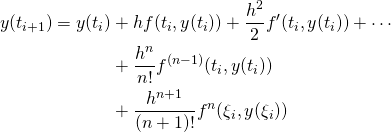
The original idea of Euler’s method can then be generalized as,
(11) ![]()
where,
(12) 
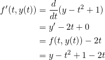
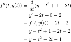
So, if we go back to the problem stated in equation ![]() , then we can write,
, then we can write,
(13) ![]()
(14) 
(15) 
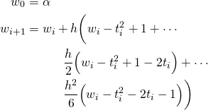
Then a third order Taylor method looks like,
(16) 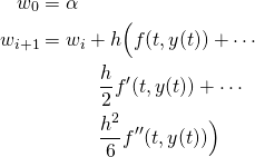
which can be expanded to,
(17) 
We can now write two Python functions to implement Taylor’s method:
def factorial( n ):
    if n == 0:
        return 1
    fact = 1
    for i in range( 1, n+1 ):
        fact *= i
    return fact

def taylor_mthd( f, a, b, N, IV ):
    h = (b-a)/float(N)                  # determine step-size
    t = np.arange( a, b+h, h )          # create mesh
    w = np.zeros((N+1,))                # initialize w
    t[0], w[0] = IV                     # set initial values
    for i in range(1,N+1):              # apply Euler's method
        T = 0
        for j in range(len(f)):
            h_factor = h**(j)/float(factorial(j+1))
            T += h_factor * f[j]( t[i-1], w[i-1] )
        w[i] = w[i-1] + h * T
    return w
And then we can calculate the second and third order Taylor method for N=10 as follows:
a, b = 0.0, 2.0
N = 10
h = (b-a)/N
IV = ( 0.0, 0.5 )
t = np.arange( a, b+h, h )

f   = lambda t, y: y - t**2.0 + 1
df  = lambda t, y: y - t**2.0 + 1 - 2*t
ddf = lambda t, y: y - t**2.0 - 2*t - 1

w2 = taylor_mthd( [ f, df ], a, b, N, IV )
w3 = taylor_mthd( [ f, df, ddf ], a, b, N, IV )
We can then plot the results as follows:
plot( t, w2, label='2nd order' )
plot( t, w3, label='3rd order' )
plot( t, y(t), label='exact' )
title( "Taylor's Method Example, N="+str(N) )
xlabel('t')
ylabel('y(t)')
legend(loc=4)
grid()
savefig( 'taylor_example.png', fmt='PNG', dpi=100 )

For N=10 the second order Taylor’s method obtains an absolute error of 0.142087, while the third order calculation obtains an absolute error of 0.0070591.
Runge-Kutta Methods
The Runge-Kutta methods are important because they allow us to achieve pretty good accuracy without having to calculate derivatives of functions, assuming those derivatives exist.
The Midpoint Method
(18) 
def midpoint_method( f, a, b, N, IV ):
    h = (b-a)/float(N)                  # determine step-size
    t = np.arange( a, b+h, h )          # create mesh
    w = np.zeros((N+1,))                # initialize w
    t[0], w[0] = IV                     # set initial values
    for i in range(1,N+1):              # apply Midpoint Method
        w[i] = w[i-1] + h * f( t[i-1] + h/2.0, w[i-1] + h * f( t[i-1], w[i-1] ) / 2.0 )
    return w

The Modified Euler Method
(19) 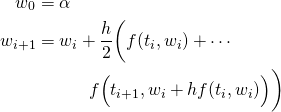
def modified_euler_method( f, a, b, N, IV ):
    h = (b-a)/float(N)                  # determine step-size
    t = np.arange( a, b+h, h )          # create mesh
    w = np.zeros((N+1,))                # initialize w
    t[0], w[0] = IV                     # set initial values
    for i in range(1,N+1):              # apply Modified Euler Method
        f1 = f( t[i-1], w[i-1] )
        f2 = f( t[i], w[i-1] + h * f1 )
        w[i] = w[i-1] + h * ( f1 + f2 ) / 2.0
    return w

Heun’s Method
(20) 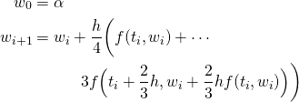
def heun_method( f, a, b, N, IV ):
    h = (b-a)/float(N)                  # determine step-size
    t = np.arange( a, b+h, h )          # create mesh
    w = np.zeros((N+1,))                # initialize w
    t[0], w[0] = IV                     # set initial values
    for i in range(1,N+1):              # apply Heun's Method
        f1 = f( t[i-1], w[i-1] )
        f2 = f( t[i-1] + (2.0/3.0) * h, w[i-1] + (2.0/3.0) * h * f1 )
        w[i] = w[i-1] + h * ( f1 + 3.0 * f2 ) / 4.0
    return w

Runge-Kutta Order Four
(21) 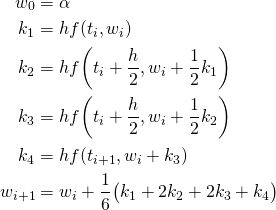
def runge_kutta_4_method( f, a, b, N, IV ):
    h = (b-a)/float(N)                  # determine step-size
    t = np.arange( a, b+h, h )          # create mesh
    w = np.zeros((N+1,))                # initialize w
    t[0], w[0] = IV                     # set initial values
    for i in range(1,N+1):              # apply Fourth Order Runge-Kutta Method
        k1 = h * f( t[i-1], w[i-1] )
        k2 = h * f( t[i-1] + h / 2.0, w[i-1] + k1 / 2.0 )
        k3 = h * f( t[i-1] + h / 2.0, w[i-1] + k2 / 2.0 )
        k4 = h * f( t[i], w[i-1] + k3 )
        w[i] = w[i-1] + ( k1 + 2.0 * k2 + 2.0 * k3 + k4 ) / 6.0
    return w

Between equations 2 and 3, you wrote “divide” where you needed “multiply.”
Derp, you’re right! Thanks!
You should also probably point out that there are a number of libraries in Python that do this for you, so that you don’t have to reinvent the wheel if you need this functionality. scipy.integrate for the well-known stuff and David Ketcheson’s nodepy for research-class Runge-Kutta solvers.
For Runge-Kutta with adaptive stepsize, see
ode23.pyunderhttps://gist.github.com/denis-bz .
it’s just for students — haven’t used it on anything real.
Nonetheless, adaptive methods can do pretty well.